Solomonoff Prior and
the Inductive Limits of Deep Learning
Abstract
In this post, I argue that large language models (LLMs), as representatives of the deep learning paradigm, are inherently incapable of achieving artificial general intelligence (AGI).
Deep learning models being inductive compressors must rely on inductive bias, a dependency highlighted by the uncomputability of Solomonoff’s universal prior.
I illustrate this fundamental limitation by constructing prior-induced adversial environments based on the ARC-AGI benchmark.
This discussion is self-contained and reintroduces all necessary concepts for clarity.
Based on A Guide to the Abstraction and Reasoning Corpus (ARC-AGI).
Table of Contents
1. Brief introduction to ARC-AGI
For all the progress made, it seems like almost all important questions in AI remain unanswered. Many have not even been properly asked yet.
- Francois Chollet
ARC-AGI was introduced in 2019 by François Chollet in his paper On the Measure of Intelligence. It remains the most challenging benchmark to date for evaluating a machine’s reasoning and generalization abilities (see Section 2, Machine Learning as an ill-posed problem).
For a more detailed introduction, refer to Section 4.1, A Guide to the Abstraction and Reasoning Corpus (ARC-AGI).
A distinctive feature of the benchmark is that most humans can solve nearly all tasks in a reasonable amount of time, but so far, no machine has yet achieved human performance, not even advanced models as Large Language Models (LLMs) and Large Reasoning Models (LRMs), which have been trained on the vast majority of high-quality human-generated data available on the internet as of 2025.
The central challenge is to build a machine that can solve these tasks efficiently in both time and computational resources. As explained in Section 3 (On General Intelligence), and Section 5 (Why Deep Learning Falls Short of AGI), any definable environment theoretically admits the existence of an “intelligent” agent. The deeper challenge, however, lies in constructing an agent that can operate effectively across arbitrary environments in practice.
At the beginning of 2025, the best approaches for solving these tasks have been discrete brute-force program search in a domain-specific language (DSL), test-time tuning (TTT) of LLMs, in particular the AIRV method, and Evolutionary Test-Time Compute.
For more in-depth explanations, refer to Section 4.2 of A Guide to the Abstraction and Reasoning Corpus (ARC-AGI).
2. Machine Learning is an ill-posed problem
Dwell on the past and you’ll lose an eye... Forget the past and you’ll lose both eyes.
— Aleksandr Solzhenitsyn
The science of data did not begin with machine learning but rather with statistics, and their respective goals are quite different. Statistics aims to collect, analyze, interpret, and present data to make informed decisions, draw conclusions, and understand patterns or relationships within data. In contrast, machine learning focuses on developing models that can learn from existing data and generalize to make predictions on new, unseen data.
Definition: (Machine Learning Problem)
Let $\mathcal{D}_{obs}:= \{ (x_1,y_1), (x_2,y_2), \ldots, (x_n,y_n) \}$ be the observed sample of I/O points from the dataset $\mathcal{D} \in X \times Y$. Machine learning aims to find a function $$f: X \rightarrow Y \quad \text{such that}\quad f(x_i) = y_i,\quad i = 1, \ldots, n.$$
More generally, given $\mathcal{D}_{obs}$, an observed sample from the joint distribution $P(x,y)$, we seek a (possibly stochastic) function $f$ that approximates the conditional distribution $P(y \mid x)$ in supervised learning, or the marginal distribution $P(x)$ in unsupervised learning.
As made explicit by the definition above, many machine learning problems are considered ill-posed, as they may lack unique or stable solutions, especially when data is limited or noisy. Furthermore, some machine learning task can be framed as inverse problems, as the goal is to infer the underlying data-generating processes $P(x,y)$ by optimizing the parameters $\theta$ of the function representing the model $f_\theta(x,y)$.
Definition: (Inverse Problem of a Model)
Consider a system that can be represented by a deterministic, parameterized function $f_\theta: X \rightarrow Y$, which we will refer to as our model. Suppose we have observed a sample of input–output (I/O) data points from this system.
The forward problem consists of computing the system’s response for a given input, i.e. evaluating the model’s output $f_\theta(x)$. In contrast, the inverse problem consists of inferring the parameters $\theta$ from observed output data $\mathcal{D}_{\text{obs}}$, such that the model with those parameters is consistent with (or generates) the observations.
Because the inverse problem is ill-posed, its solutions are not unique and are often only locally optimal. Therefore, to have any hope for an algorithm to effectively navigate the space of solutions, we must constrain it to help guide the algorithm. This is typically achieved by introducing prior knowledge or an inductive bias.
Principle 1: Any algorithm that solves an ill-posed inverse problem must effectively implement some form of prior or regularization.
Example 3: This prior knowledge is usually introduced by the choice of the algorithm the hyperparameters:
-
(Regression) There are infinitely many polynomials that can fit a finite set of points via Legendre interpolation, but high-degree polynomials often overfit the data. Therefore Bias, such as preferring lower-degree polynomials is introduced through regularization, guiding models toward simpler, more generalizable solutions.
-
(Clustering) In K-means clustering, the number of clusters must be specified in advance. This constraint prevents arbitrary or meaningless groupings and ensures the problem is well-posed.
-
(Decision Trees) Similarly, decision trees use constraints like maximum depth or minimum samples per leaf to avoid overly complex trees that memorize the training data. These biases help the model generalize better by restricting its capacity.
From a physicist’s point of view, when considering machine learning as a field of observation and modeling, we have argued the necessity of inductive bias or prior knowledge to solve such problems. From a mathematical perspective, however, we must ask: what does it mean to solve these problems, and can we reach a consensus on the definition of intelligence within this framework?
For sake of completness, let us rephrase the problem: let $P(x,y)$ be a probability distribution defined on the space $\mathcal{D}$, from which we can only observe a subset, the observed sample $\mathcal{D}_{obs}$. The goal is to infer the “best” generative mechanism of the probability distribution of the whole space $\mathcal{D}$, from the limited knowledge of the observation space!
The ability to correctly predict outcomes on unseen data drawn from a partially observed distribution is often regarded as a hallmark of intelligence. More precisely, it is the reason why the field is called machine learning: the ability to take optimal actions in unseen environments without being explicitly programmed to do so.
For this reason, when developing such a model, we usually split the observed data into training $80\%$, validation $10\%$, and test $10\%$ subsets. In practice, such a distinction makes sense as we are bounded by our limited observations. Which is why,
Lemma 2: The performance of a machine learning models depends highly on:
- The complexity of the underlying probability distribution $P(x,y)$.
- The size of the observed sample $\mathcal{D}_{obs}$.
- The “difference” between the training, and test distributions.
How surprising is it that the distributions generating the training and test samples may differ, and that both can also deviate from the true underlying probability distribution? What explains this seemingly unintuitive behavior?
Bounded by our being, our observations are constrained by the limits of our perception and measurement. Consequently, we must rely on a sampling procedure, whether it is from a physical experiment or from a mathematical model. Although sampling may appear trivial at first glance, the design and interpretation of sampling procedures constitute one of the most complex and fundamental problems in statistics and the sciences.
A striking historical example comes from the Manhattan Project (Nuclear Weapon), where scientists confronted the impossibility of analytically solving high-dimensional integrals had to approximated them through repeated random sampling, giving rise to what we now call the Monte Carlo method. This illustrates how fundamental sampling is, not only for scientific discovery at the highest stakes, but also for modern machine learning, where the reliability of models depends on how well our sampled data represents the underlying distribution.
Example 4: Given a sampling procedure, the underlying distribution can be quite different to the training/test ones.
Therefore, the performance of a model trained on data sampled from the underlying distribution depends not only on the amount of data required to generalize within the training distribution, but also on its ability to handle distributional shifts between training and test sets, thereby ensuring robustness and adaptability in previously unseen scenarios.
Definition: (Out-of-Distribution Generalization)
Out-of-distribution generalization refers to the ability of a machine learning model to perform well on test data whose distribution differs from that of the training data.
For the sake of simplicity, we will not provide a formal definition of distance between probability distributions, nor analyze in detail how training and testing distributions may differ. Readers interested in this topic may consult common measures such as the Kullback–Leibler divergence or the Wasserstein distance.
Having defined out-of-distribution (OOD) generalization as a measure of model intelligence, we may now ask, following the three crucial points of Lemma 2, how the amount of available data influences this capability.
Consider the case where a model is provided with K examples drawn from a given distribution: if it succeeds in inferring the underlying structure and generalizing from this limited sample, the process is known as K-shot learning.
Definition: (K-Shot Learning)
\(K\)-shot learning is a machine learning paradigm in which a model must correctly recognize or classify new concepts given only \(K\) training examples per class, often with \(K\) being very small (e.g., one or few).
Thus, the highest level of model intelligence can be regarded as the combined ability to achieve both one-shot (or few-shot) learning and out-of-distribution (OOD) generalization.
This is precisely the capacity that the ARC-AGI benchmark is designed to evaluate, making it one of the most significant benchmarks proposed to date.
3. On General Intelligence
The meaning of a word is its use in the language.
— Ludwig Wittgenstein
The promise of artificial general intelligence (AGI) is to develop a general algorithm or model capable of solving a wide range of problems without relying on prior knowledge (including hyperparameters and model selection; see Section 2).
To not encounter a paradox when defining AGI, we have to cojointly define artificial super intelligence (ASI) as an algorithm capable of meta reasoning, i.e. to reason about itself and therefore of intelligence more broadly. Such a distinction is necessary; without it, we risk running into paradoxes.
Most, if not all, mathematical problems require a space and a metric in which the problem is embedded. Without such a formal space in our discussion, it becomes impossible to rigorously speak about the proprieties of the considered object, such as optimality or uniqueness. This opens the door to paradoxes such as infinite regress, fixed-point pathologies of self evaluation $\ldots$
Such a discussion is related to our philosophical stance on language. Do words have meaning only in context as in Wittgenstein or Saussure sense, or do they possess an absolute, intrinsic meaning as in Plato’s view of eternal forms?
By analogy, we can pose the same question with respect to intelligence. Is intelligence fundamentally context-dependent, in the sense that an algorithm’s performance is meaningful only relative to a specified evaluation space and utility functional? In this view, the paradox dissolves, since one can define a supremum (or maximum, if attained) within this space, as is done in the Universal Intelligence Measure Legg & Hutter, 2007, which evaluates agents as weighted averages of performance across computable environments.
Alternatively, one might suppose that “intelligence” exists in some absolute medium. In that case, paradoxes such as infinite regress re-emerge unless the ambient space and its associated metric are rigorously defined and one can prove the existence of a well-defined maximizer. This connects directly to results such as the No Free Lunch theorems Wolpert & Macready, 1997, which formalize the impossibility of universally optimal performance absent assumptions about the problem distribution.
Definition: (A solvable problem)
A problem $p$ is a set of ordered pair $\{(Q,A)\}$ where each $Q,A$ are instances describable by a language game. A problem is solvable if there exists an algorithm $a$ such that $a(x)=y$ for all $(x,y) \in P$.
Example 4: Consider the following problem $p:={ \text{addition of two elements} }$. Such a problem is describable by language game, example of pairs are $(2+2,4)$ or $(3.14 - 8, -4.86)$.
The two following algorithms are solution, $a_1$:
def f(a:element, b:element):
  return a+b
or $a_2$:
def f(a:element, b:element):
  return 5 + a - 3 + b -2
Within such a framework, one can define both a metric and a notion of optimality. Drawing from Algorithmic Information Theory (AIT), optimality is naturally characterized using Kolmogorov complexity: the shortest program that solves a given task. For further discussion, see Section 5.
Definition: (Solver)
Let P be the set of problem admitting at least one solution and $P' \subset P$ a subset. The function S is said to be a solver of $P'$ if $$S: P \rightarrow A \quad \text{such that}\quad S(p)\in A_p \quad \forall p \in P'.$$ Where $A_p$ is the set of algorithm solving the given problem p.
Definition: (General Intelligence)
A solver is said to have general intelligence if the subset on which it is a solver is P itself.
Definition: (Super Intelligence)
We do not restrict ourselves to problems describable by a language game, but also consider meta-problems, which may include solvers themselves. A solver of such a problem is called a meta-solver. A meta-solver is said to possess superintelligence if it has meta-general intelligence, which is defined analogously to general intelligence but for this broader class of problems.
4. Deep Learning models are compressors
The problem of learning is the problem of finding regularities in data, and regularities are precisely what can be used to compress the data.
— Ray Solomonoff
Deep Learning can be elegantly summarized as follows:
Principle: [Deep learning]
Deep learning models perform feature extraction by learning compressed representations of the data through nonlinear mappings, guided by the dynamics of the loss function.
This principle has a significant consequence, which can be illustrated with a simple example.
Example 4: A simple perceptron or a convolutional neural network (CNN) trained to classify cats versus dogs will learn representations tailored specifically to that task. Features irrelevant to minimizing classification error, such as background color, are typically ignored. Consequently, the model’s internal representations are optimized exclusively for the training objective, rather than for capturing information beyond it.
Three key properties of deep learning models can be summarized as follows:
Proposition: [Deep learning Models are Universal Approximators].
Cybenko 1989 showed that Under suitable conditions, neural networks are dense in the space of continuous functions: for any function $f$ defined on a compact set and for any $\epsilon > 0$, there exists a neural network $\phi$ such that \[ \sup_{x} | f(x) - \phi(x) | < \epsilon . \]
Proposition: [Deep Learning Models are non-picky learners].
Zhang 2016 showed that sufficiently overparameterized deep learning models, trained with stochastic gradient descent (SGD), can achieve zero training loss regardless of the structure of the data. This holds even when labels are randomly permuted or when the inputs consist entirely of noise.
Proposition: [Deep Learning Models are Weak OOD Generalizers].
Let \(p \in \mathcal{P}\) denote a symbolic reasoning task (e.g., pointer value retrieval). Empirical studies by Zhang et al. (2022) show that deep neural networks trained on \(p\) with data distribution \(\mathcal{D}_{\text{train}}\) often fail to generalize when evaluated on an out-of-distribution \(\mathcal{D}_{\text{test}} \neq \mathcal{D}_{\text{train}}\). However, Boix-Adserà et al. (2024) demonstrate that transformer architectures trained with stochastic gradient descent (SGD) achieve \[ 0 < \mathbb{E}_{x \sim \mathcal{D}_{\text{test}}}[ \mathbf{1}\{ f_\theta(x) = p(x) \}] \ll \mathbb{E}_{x \sim \mathcal{D}_{\text{train}}}[ \mathbf{1}\{ f_\theta(x) = p(x) \}], \] i.e., non-trivial but suboptimal generalization performance beyond the training distribution.
It is further observed that such positive OOD generalization occurs for transformers, but fails for simpler architectures such as multi-layer perceptrons (MLPs), which yield performance indistinguishable from chance under the same conditions.
Given that the abilities of deep learning models are strongly correlated with their compression capabilities, their empirical efficiency provides supporting evidence for the following principle:
Hypothesis: (Manifold Hypothesis).
Real-world data are concentrated on (approximately) low-dimensional manifolds embedded within high-dimensional spaces, allowing for compression that preserves the information necessary for generalization.
This naturally motivates a deeper question:
Hypothesis: [Universal Lossless Representation].
Does there exist a universal representation medium \(C\) that is lossless across all tasks, in the sense that it preserves all potentially relevant information required for generalization?
We argue in the negative: reliance on compression alone can hinder generalization. In particular, ARC-AGI provides a practical example of an adversarial Solomonoff environment, illustrating the inherent tension between computability and expressivity.
5. Glimpse of Induction Theory
That the sun will not rise tomorrow is no less intelligible a proposition, and implies no more contradiction, than the affirmation that it will rise.
— David Hume
The problem of induction has been debated philosophically since the 1800s by Hume to the 2000s by Popper. Their view about it as a scientific method was rather critical as it did not rest on any rational justifications. For this reason, Popper strongly advised to use conjectures and refutations as the engine of science.
Definition: [Induction]
Induction is the problem of inferring rules (or hypotheses) from observed data to predict unobserved data.
Hume’s challenge to the theory is that we have no rational guarantee the future will resemble the past.
The Bayesian framework does not solve this issue but offers a pragramtic answer to a simplified problem by embedding it into a mathematical framework.
Principle: Bayesian Probability Theory
What is the optimal way to update my beliefs given new information?
This relies on two fundamental assumptions,
Lemma 5: Prior of Bayesian reasoning
- A predefined hypothesis class \(\mathcal{H}\).
- Prior probabilities \(\pi(h)\) assigned by the experimenter.
Given a hypothesis $h \in \mathcal{H}$ with prior $P(h)$ and evidence $x$, beliefs are updated by
Theorem: [Bayes Theorem]
For any hypotheses \(h\) and evidence \(x\), the posterior probability is defined as, $$ P(h\mid x)=\dfrac{P(x\mid h)P(h)}{P(x)} $$
In the 1960s, observing both the strength of Bayes its limitations imposed by priors, Solomonoff asked himself:
Definition: [Solomonoff Hypothesis]
Can there exist a universal prior that depends on no subjective domain assumptions?
His key insight was to treat every computable model, which is every program that could generate the observations, as a candidate hypothesis, weighted inversely by its complexity. More precisely he defined $\mathcal{H}$ as the set of all computable programs and assigned probability to its elements relative to their simplicity.
Definition: [Kolmogorov Complexity]
For a universal Turing machine \(U\), the Kolmogorov complexity of a finite string \(x\) is
\[ K_U(x) \;=\; \min_{p:\, U(p)=x}\; |p|, \]
the length of the shortest program that outputs \(x\).
The following lemma shows that the derived results are independant of the choice of the Turing Machine, which is why we avoid to define it explicitly.
Lemma:
For any universal machines U and U', there exists a constant $c$ such that for all strings $x$: $$ |K_U(x)-K_{U'}(x)| \leq c. $$
Borrowing Kolmogorov notion of complexity we can finally introduce Solomonoff Prior.
Definition: [Solomonoff Prior]
The universal a priori probability of a string \(x\) is
\[ P(x) \;\propto\; \sum_{p:\, U(p)=x} 2^{-|p|}, \]
summing over all programs \(p\) that output \(x\) on \(U\).
This extends Bayes’ rule to the full space of computable hypotheses, building in Occam’s Razor (prefer simpler explanations) and Epicurus’ Principle (consider all consistent explanations).
At the ideal limit, Solomonoff induction predicts by mixing over all programs that could generate the data, giving greater weight to shorter ones. This ties generalization to compression: shorter descriptions tend to predict better. But the Solomonoff prior is incomputable, it requires summing over all programs, so practical learners must rely on specific inductive biases (prior) as explained in Section 2 (Machine Learning is an Ill-posed Problem).
Definition: [Computable]
A method is computable if a finite, effective procedure (e.g., a program on a universal Turing machine) outputs a result in finite time for any valid input.
Definition: [Expressive]
A hypothesis class is expressive to the extent it can represent (or approximate) a broad set of functions/environments; maximal expressivity approaches “all computable mappings.”
In the following Section (Why Deep Learning Falls Short of AGI), we will exploit the implicit use of prior used by LLM to construct an adversarial environment, highlighting the inherent shortcomings of deep learning, and more generally inductive reasoning for our definition of artificial general intelligence.
6. Why Deep Learning Falls Short of AGI
Without prior assumptions about the problem, no learning algorithm can be expected to outperform any other.
— David Wolpert and William Macready
6.1 Framework
From the previous section:
- The Solomonoff prior is incomputable; practical inductive learning must rely on inductive bias.
- Deep learning’s main inductive bias assumes compressible structure (e.g., the Manifold Hypothesis).
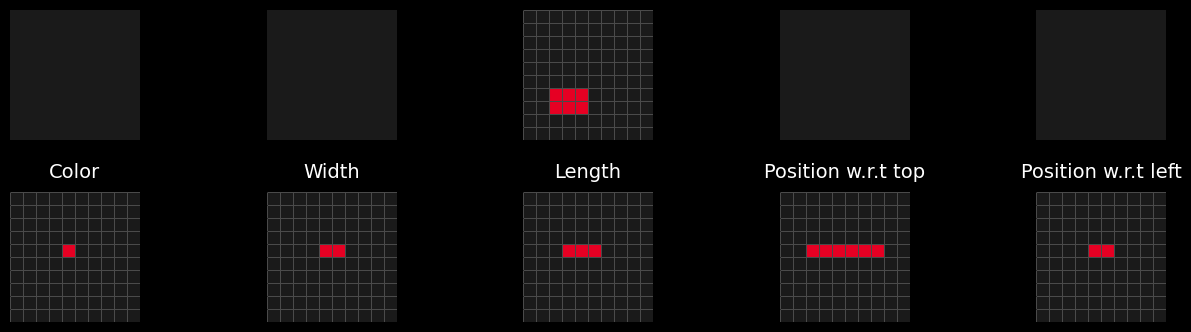
The beauty in ARC-AGI is that even if all the tasks are simple I/O grids, the framework offers such an extremely rich universe, that even if they share the same format, the inductive bias required to solve two tasks can have nothing in common.
The clearest and most striking evidence for this comes from the Test-Time Tuning paradigm that emerged in ARC-AGI 2024. It was observed that, regardless of model size, the model quickly saturated on a given task and could not transfer its learning to a different one.
We believe this limitation arises from the implicit biases required for inductive learning to occur.
Framework:
In our framework each task $T$ can be though of as an environment of the universe and the model $f_\theta$ as a solver, where $\theta$ is the parameter we optimize for each task.
Simple problem (environment learning): Find a model that can saturate any environment,
\[\forall\,T\ \exists\,\theta:\ \operatorname{Performance}(f_\theta,T)\ \text{is high},\]Hard problem (universe learning): Find a model that can saturate the universe,
$$ \exists\,\theta\ \forall\,T:\ \operatorname{Performance}(f_\theta,T)\ \text{is high}. $$
The proof principle rests on the No Free Lunch theorem:
Theorem: [No Free Lunch]
Any performance gain on one class of problems is offset by a loss on another, when averaged over all problems.
Here is the core tension:
- Maximally expressive systems (Solomonoff induction) are incomputable.
- Maximally computable systems (deep learning) restrict expressivity and fail outside their inductive bias.
Theorem: (Computability–Expressivity Trade-off)
No algorithm can be both universally computable and maximally expressive.
Consequently, every practical learner faces environments where it fails to generalize.
6.2 Natural Language as a Mathematical Operator of Information
To avoid combinatorial explosion, both biological and artificial neural systems process information through intermediate, compressed representations. As the Human language has been improved for over thousands of years it has acquired a unique kind of richness, which allow us to use it for a major part of our reasoning process.
The very quality that gives words their strength is also their weakness. In Wittgenstein’s view, words derive meaning only in relation to one another. To carry meaning, they must describe; yet in doing so, they constrain, and thus compress.
Every sentence in any language exemplifies one of the most profound phenomena of complex systems: emergent behavior. First introduced by Philip W. Anderson in More Is Different.
Definition: [Emerging Behavior]
A system is emergent when its collective behavior cannot be reduced to or predicted from the properties of its parts alone.
The system as a whole becomes more than the sum of its components.
Principle: [Language Meaning is emergent]
Individual linguistic units are descriptive tools (compressors); in composition, they become expressive systems.
Models constrained to reason within this compressed space inherit the same paradox: their capacity to generalize is limited by their inability to transcend the very compression that enables them, unless they grasp the totality of emergent phenomena that manifest within every sentence.
Example: Word: object in the gridspace.
In the grids space, a compressed representation of a connected set of pixels can be the natural language word 'object'. If our goal is, as a deep learning model, to quantify the presence of objects in a grid, this lossy representation is sufficient and more optimal than to incorporate all the information from the grid. This representation is a "projection" as it will not offer us the ability to return to the initial task as it it lossy.
Even if language as a representation space is lossy for information, its basic units have well-defined mathematical proprieties.
Lemma: The language space is a quotient space.
Let \( I \) denote the space of information where the grids reside, and let \( H: I \to L \) be a function mapping each information instance to its linguistic representation in the language space \( L \). Then, \( L \) can be viewed as a quotient space of \( I \), where each element of \( L \) corresponds to an equivalence class of information instances that share the same linguistic description.
Example: Mathematical properties of the word object.
Continuing the previous example: any invertible transformation of the grid, such as a rotation, preserves the notion of “object.” Hence, all grids related by such transformations belong to the same equivalence class, represented by the word “object.” The word thus corresponds to an equivalence class under a set of invariances.
The advantage of working within an equivalence class is that it simplifies reasoning and proofs by abstracting away irrelevant variations. The disadvantage is that it forces to use to rely on inductive bias to choose the representations.
Thought Experiment: [Pitfall Inductive Reasoning]
No compression, no generalization; too much compression, flawed generalization.
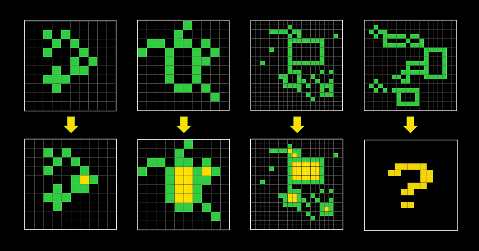
Consider a 10x10 grid containing black pixels and a 2x3 red rectangle positioned two pixels from the right border and two pixels from the top border. If the logic is to output the number of objects in the grid, then in the description we must specify the presence of an object in the grid. If the task is to output the color, we must specify the color of the object. Similarly, if the task is to determine the width or height of the objects, we must specify their dimensions. If the task requires the distance relative to the left, top, bottom, or right borders, we must also include the spatial position. Therefore, a naive, exhaustive description is highly suboptimal. As the task becomes more complex, its length grows exponentially longer. To manage this, we unconsciously abstract certain characteristics and decide to focus on a subset of the information. This abstraction is achieved by comparing the set of puzzles in a task to see what can be abstracted to reduce some degrees of freedom, for instance, by omitting the explicit mention of spatial position when it is not relevant to the task. This approach results in a quotient representation of the information. For example, describing the object as a "red rectangle" implicitly assumes position invariance and indicates that rotating the object does not alter its description. Through this process, we interact with the task more effectively by prioritizing relevant features and abstracting unnecessary details.
This freedom of task construction forces us to encode all the information in a lengthy intermediate reasoning representation.
6.3 Experiments
Structure:
LLMs generate internal feature representations at each layer. These representations evolve as information flows through the network capturing progressively more abstract patterns of the input.
Each layer acts as a compression mechanism: it filters and condenses the information of the previous layers, preserving only what is useful for the model’s objective. This compression reflects how the model encodes the essential structure of the task while discarding redundant or noisy details. In a similar fashion to adopting a more elaborate vocabulary to describe (and therefore to disregard) information. As demonstrated in the Thought Experiment such a process is necessary to avoid combinatorial explosion. In the following experiments, we aim to show this behavior.
Steps:
- Consider the complete set of tasks, each composed of training and test examples.
- Retain the subset of tasks for which the LLM successfully predicts the test output given the input and training examples
- Using the equivalence established in A Guide to the Abstraction and Reasoning Corpus (ARC-AGI) between a task and its corresponding input generator–solver pair, generate a collection of approximately 100 new test inputs and solve them with the generator.
- Retain the corresponding subset of these test–training examples on which the model failed and observe the internal representations of the LLM across its layers.
- (Ideally) develop an algorithm capable of identifying adversarial test inputs that emerge as a result of representational compression within the LLM.
In simpler terms, the hypothesis is that the LLM may not explicitly distinguish between closely related concepts, which are the product of multiple layers activations. For example, “rectangle” and “square” if doing so provides little informational gain. Instead, for efficiency (in an information-theoretic sense), it might internally represent both as the higher-level category “quadrilateral.” The goal is to demonstrate that this kind of conceptual compression occurs between certain layers (say, between layers n and p), by comparing internal representations across tasks and inputs that probe different levels of abstraction.